The Spring Predictability Barrier: we’d rather be on Spring Break
It’s that time of year again when ENSO forecasters stare at the latest analysis and model forecasts and shake their heads in frustration. Why? We’re in the heart of the so-called “Spring Predictability Barrier,” which is when the models have a harder time making accurate forecasts. It’s like trying to predict the next episode of Mad Men based on the tiny amount of detail given in the “as seen on the next episode” clips. As we know from Tom’s posts on verification (here, here, here), there are many ways to measure the accuracy, or skill, of seasonal climate predictions. Here, we will focus on just one measure (1), but there are other ways to gauge the spring barrier.
What is the Spring Barrier?
Is the Spring Barrier like a brick wall? In other words, do we smack right into it and cannot see or predict anything beyond it? No, not really. It is more like a lull or a valley in ENSO forecasting accuracy. After the spring (or the autumn for our friends in the Southern Hemisphere), the ability of the models to predict becomes increasingly better. Keep in mind that, in general, the skill of the models get better the closer you get to the period of time you are predicting. If you want to know whether it is going to rain, you are usually better off using a prediction the day before than you are a week out. The same is true in seasonal climate outlooks. However, during the spring, even making an ENSO forecast for the coming summer is pretty difficult.
April 2015 is almost over, and so how useful have the model forecasts been if we want to predict ENSO for the May-June-July (MJJ) season (2)? As you will see, the Spring Barrier is the climate forecaster’s equivalent of mayhem. In a perfectly predictable world, we would be able to predict 100% of ENSO variability. But statistical models (3) barely register a pulse, describing almost none of the fluctuations in ENSO during the MJJ season. State-of-the-art dynamical model (4) don’t fare much better, only accurately predicting about less than a third (33%) of ENSO variability in the MJJ season. So, even for the closest period coming up, ENSO forecasters can’t say a lot about it!
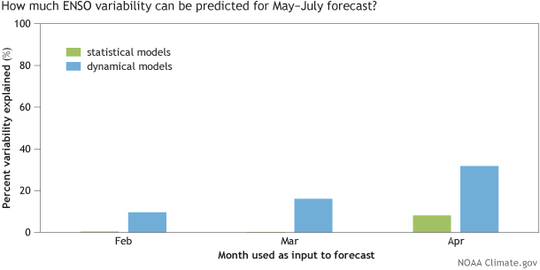
The skill (or forecasting ability) of model runs based on February, March, and April observations to predict the May-July (MJJ) average value in the Niño-3.4 SST region (ENSO). Results shown here are an average correlation coefficient from each of the 20 models between 2002-2011 (data used from Barnston et al, 2012). Percent Explained Variance (%) is calculated by squaring the correlation coefficient and multiplying by 100 (see footnote #1). Models that explain all ENSO variability would equal 100%, while explaining none of the ENSO variance would equal 0%. Graphic by Fiona Martin based on data from NOAA CPC and IRI.
Now let’s shift our attention to making an ENSO prediction for the coming winter season (for the November-January seasonal average). How useful are the models? Well, if you’re running a model using October data as input, then you’re in pretty good shape as you can expect close to 90% of the winter ENSO fluctuations to be predicted. In terms of lead time, that’s the same horizon as a forecast made in April for May-June-July (MJJ), and yet there is a huge difference in forecasting ability (5).
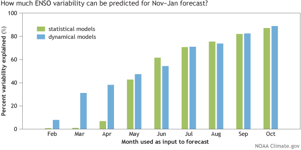
The skill (or forecasting ability) of model runs based on February-October observations to predict the November-January (NDJ) average value in the Niño-3.4 SST region (ENSO). Results shown here are an average correlation coefficient from each of the 20 models between 2002-2011 (data used from Barnston et al, 2012). Percent Explained Variance (%) is calculated by squaring the correlation coefficient and multiplying by 100 (see footnote #1). Models that explain all ENSO variability would equal 100%, while explaining none of the ENSO variance would equal 0%. Graphic by Fiona Martin based on data from NOAA CPC and IRI.
However, hope slowly grows as we emerge from the spring. In particular, models run based on May data are getting close to explaining half of the coming winter variability, which isn’t shabby.
But, still, predictions are still far from assured. Using July and August data, about three-quarters of the winter ENSO fluctuations are predicted by the models. So while forecast “surprises” are becoming less frequent, they still lurk around.
Overcoming the Spring Barrier?
So, why is the accuracy of the models so bleak during the spring? Is there reason to believe that more model development will improve upon the low skill we see during the spring? While there are many ideas on why the spring barrier exists, there are no definitive culprits (Webster and Yang, 1992, Webster, 1995, Torrence and Webster, 1998, McPhaden, 2003, Duan and Wei, 2013).
One of the reasons that the spring barrier is said to exist is because spring is a transitional time of year for ENSO (in our parlance, signals are low and noise is high). The spring is when ENSO is shifting around— often El Niño/La Niña events are decaying after their winter peak, sometimes passing through Neutral, before sometimes leading to El Niño/La Niña later on in the year. It is harder to predict the start or end of an event than to predict an event that is already occurring. There is also weaker coupling between the ocean-atmosphere in the spring due to a reduction in the average, or climatological, SST gradients in the tropical Pacific Ocean. However, for various reasons, these factors don’t fully explain why we see lower skill (6).
Illustration by Emily Greenhalgh, NOAA Climate.gov.
One “clue” for the barrier lies in the fact the dynamical models perform better compared to the statistical models during the spring (see figure above: the blue bars are larger than the green bars). In fact, just during the last decade, dynamical models have slightly edged statistical models in their overall ENSO forecast ability because of their improvement during the spring (Barnston et al., 2012). During the other seasons, running a statistical or dynamical model gives you about the same amount of ENSO forecast skill.
What is special about dynamical models during the spring? One of the attributes of dynamical models is that they are run more frequently using the most recent observed data as input. Many statistical models are built on monthly or seasonal (3-month) average data, so by comparison, are receiving inputs that are relatively older. Dynamical models also ingest a lot more observations (such as the subsurface ocean) using complex data assimilation schemes. These qualities may allow dynamical models to “see” better and potentially lock onto potentially important changes that occur during the spring. But keep in mind this increased skill is relative to the statistical models-- the dynamical model skill is still low overall.
As Eric Guilyardi wrote in his blog post last week, there is room to improve models by better understanding their errors and improving the assimilation of observational data. Potentially, with more research and development, we will see the models become more skillful during the spring. Until then, ENSO forecasters would rather be on spring break.
Footnotes:
(1) As a first step, we calculate the “correlation coefficient” or the Pearson’s correlation coefficient. We also introduced this concept in Tony’s blog post discussing the ENSO skill over the past couple of years. The correlation coefficient ranges between 0 (no skill) and -1/+1 (perfect skill). However, in the figures above, we put it in terms of “explained variance,” by squaring the coefficient and multiplying by 100. Explained variance can range from 0% to 100%. 0% means that the models describe none of the variability of the ENSO index (the wiggles or ups and downs in the time series). 100% means that the models predict all of the fluctuations in the ENSO. So, ideally, want to see 100% variance explained even though that will never happen because our world is not perfectly predictable.
(2) We use data gathered during a 10-year period of operational model runs, which are presented on the IRI/CPC plume of Niño-3.4 SST index predictions (Barnston et al., 2012). Un-gated copy is available here.
(3) Statistical models: computer models that predict how current conditions are likely to change by applying statistics to historical conditions. Physical equations of the ocean and atmosphere are not used. These models can be run on a small desktop computer.
(4) Dynamical models: computer models that predict various oceanic, atmospheric, and land parameters by solving physical equations that use current “initial” conditions as input. State-of-the-art dynamical models must be run on high-performance supercomputers.
(5) Because of the limited length of the operational model runs, we expect that the 95% level of significance isn’t achieved until the explained variance is greater than ~45% (based on 9 degrees of freedom and using the sampling theory of correlations). Therefore, there is a fair chance that values not reaching that threshold may be randomly achieved and therefore are not particularly meaningful.
(6) In the opinion of the author and some of her colleagues, there is a bit of a chicken-egg problem by arguing that lower skill of the models is due to the transitional nature of ENSO or the low signal-to-noise ratio in the spring. Low predictability and low signal-to-noise go hand-in-hand. One does not cause the other. Also, the fact that the climatological SST gradient is at a minimum during the spring doesn’t clearly explain why ENSO -- which is a departure from climatology (or anomaly) -- would also be impacted (and the opposite should be true in the autumn when the SST gradient is maximized-- yet ENSO peaks during the winter).
References:
Anthony G. Barnston, Michael K. Tippett, Michelle L. L'Heureux, Shuhua Li, and David G. DeWitt, 2012: Skill of Real-Time Seasonal ENSO Model Predictions during 2002–11: Is Our Capability Increasing?. Bull. Amer. Meteor. Soc., 93, 631–651.
Duan, W. and Wei, C. (2013), The ‘spring predictability barrier’ for ENSO predictions and its possible mechanism: results from a fully coupled model. Int. J. Climatol., 33: 1280–1292. doi: 10.1002/joc.3513
McPhaden, M. J. (2003), Tropical Pacific Ocean heat content variations and ENSO persistence barriers, Geophys. Res. Lett., 30, 1480, doi:10.1029/2003GL016872, 9.
Torrence, C. and P. J. Webster, 1998: The Annual Cycle of Persistence in the El Niño-Southern Oscillation. Q. J. Roy. Met. Soc., 124, 1985-2004.
Webster, P. J. , 1995: The annual cycle and the predictability of the tropical coupled ocean-atmosphere system. Meteor. Atmos. Phys., 56, 33-55.
Webster, P. J. and S. Yang, 1992: Monsoon and ENSO: Selectively Interactive Systems. Quart. J. Roy. Meteor. Soc., 118, 877-926.
Comments
April peak for ENSO conditions
I simply wanted to write down
Spring 2023
It's February 2023, and I see (from reading Emily Becker's post today, which had a link to this one) that the probabilities for next fall and winter range from a weak La Niña to a strong El Niño. So, I guess the uncertainties popping up now are part of this.
You got it!
You got it!
How can April ENSO forecast skill for NDJ exceed for MJJ?
Interesting article, but...
In the first chart, an April Dynamic model forecast for MJJ ENSO has about 33% skill as discussed in text. In the second chart, April dynamic model skill for NDJ is higher, ~ 38%. How can a forecast for 3-month period starting 7 months later be more skillful than a forecast for the closest 3-month period starting in 1 month?
The model set is the same for both charts "Results shown here are an average correlation coefficient from each of the 20 models between 2002-2011 (data used from Barnston et al, 2012)."
It would be interesting see a third chart that repeats the second chart, but showing forecast skill for MJJ based on August, Sept.... April input data.
Very good question... since…
Very good question... since you seem interested in the particular details of the skill, I would recommend a few papers to read:
https://link.springer.com/article/10.1007/s00382-017-3603-3
Figure 6 here shows correlation for all lead times and target months (not seasons but think that is ok). I will work off this figure in my explanation below:
https://journals.ametsoc.org/view/journals/clim/37/4/JCLI-D-23-0406.1.xml
Look at the models with particularly deep spring barriers... let's look at the NASA GEOSE2S model for instance. For instance look at May at lead=0 (this is both the start and target month), the skill is pretty high (deep red). Then, if we want to stick to May starts, as you advance to the June target along the diagonal (June target, lead=1), the skill drops as you get into those summer targets (paler color). Then as you continue to advance, up the diagonal to the winter starts, the skill increases again. This is just one model and I would argue that there is a fair bit of sampling variability on records as short as the ones we examine (so 33% and 38% are probably not significantly different from each other). But it does articulate a point that is evident in some of these models, which is that there is lower skill for forecasts made in the spring for the near term, upcoming seasons and there is a very tiny bit of a rebound as you get through that period. This is also something that Jiale Lou et al. noticed when he looked at multi-year ENSO predictions (see discussion under "seasonal variations of ENSO skill"):
https://www.nature.com/articles/s41612-023-00417-z
He writes "The skill minimum might therefore reflect temporarily lower boreal summer signal-to-noise ratios rather than a barrier to skill at longer leads." Which is something to consider when studying this data. Anyway great question!
Comments have been disabled on this article