Other Climate Patterns that Impact U.S. Winter Climate
While the focus of this blog is ENSO, there are other important climate patterns that impact the United States during the Northern Hemisphere winter season. We often focus on the winter season because that is the time of year many climate patterns are most prominent, and in the case of ENSO, this is the season when impacts are most predictable (1). In this post, we will define some of these other patterns and then in a subsequent post in August, we will discuss how much these patterns contribute to U.S. winter climate predictability relative to ENSO.
Long-term Trends
A major non-ENSO climate influence, which is particularly important for seasonal temperature, is long-term trends or climate change. We commonly define climate anomalies in terms of deviations from the average, or normal, climate over a recent 30-year period (e.g. the 1981-2010 period). In our gradually warming climate, most recent years are warmer than the recent 30-year average, so a winter forecast for above average temperatures can be skillful regardless of the ENSO state.
For most of the U.S., temperature is trending upward, most strongly in the Southwest and many of the northern states, and most weakly in part of the Southeast (Livezey and Timofeyeva 2008). Figure 1 shows the geographical pattern of the rate of warming over the country for the January-March season. Other seasons have somewhat slower overall warming rates, and with some variation in pattern details.
It should be noted that trends do not continue smoothly year after year. So there are some years, or even decade-long periods, that do not show a continuation of a trend that had been in progress: climate trends emerge when we look at data for a long period of time (see Fig. 2). Trends in precipitation are comparatively weaker and more variable geographically and seasonally than trends in temperature.
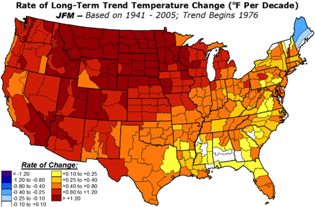
Temperature trend for the January-March season (degrees F per 10 years) between 1976 and 2005. Image credit: NOAA Climate Prediction Center.
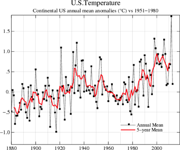
Annual average temperature anomaly over the continental U.S. with respect to the 1951-1980 period (black line), and the average of the 5 years centered on the given year (red line). This older 30-year reference period is used to accommodate the very long (134-year) analysis period. Image credit: NASA/GISS.
The North Atlantic Oscillation (NAO)/ Arctic Oscillation (AO)
Another major non-ENSO influence on winter climate is an atmospheric pattern called the North Atlantic Oscillation (NAO; Wallace and Gutzler 1981). The NAO is primarily centered over the North Atlantic Ocean but extends over Europe and the eastern US (more information here). Figure 3 illustrates the middle-atmosphere pressure pattern representing the positive NAO phase. This pressure pattern aloft would correspond to a similar pattern at the surface. The NAO is considered the regional manifestation of a hemispheric-wide pattern called the Arctic Oscillation (AO; Thompson and Wallace 2000), which is related to the polar vortex. Figure 4 shows the surface pressure pattern of the AO (which would look similar at higher levels in the atmosphere).
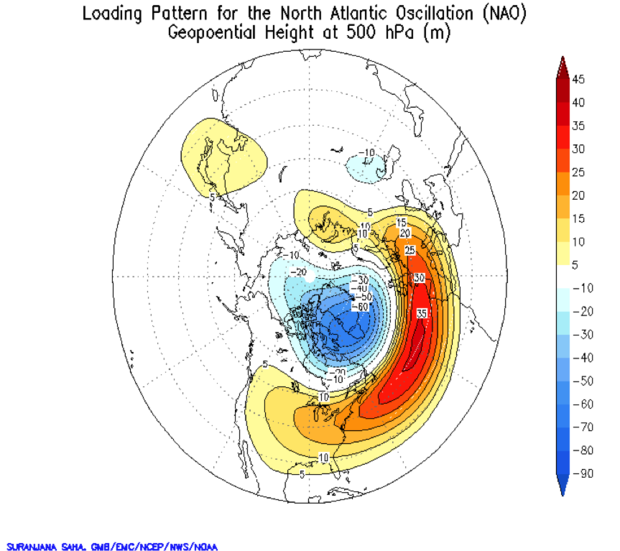
Map showing upper atmospheric pressure anomaly pattern of the North Atlantic Oscillation in its positive phase, using the statistical technique of rotated principal components analysis, which defines typical preferred anomaly patterns. The units are height (meters) of the 500mb pressure surface (higher heights indicate higher pressure at a given altitude above the surface). Image credit: NOAA Environmental Modeling Center.
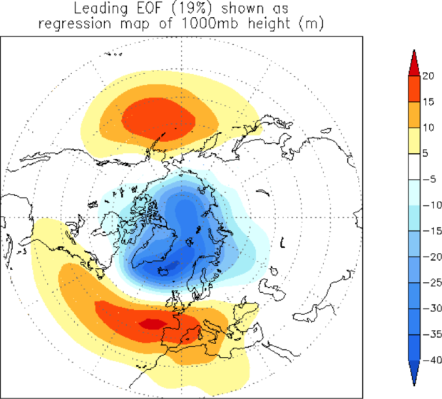
Map showing surface pressure anomaly pattern of the Arctic Oscillation in its positive phase, using the statistical technique of unrotated principal components analysis, which is another way to define typical preferred anomaly patterns. The units are height (meters) of the 1000mb pressure surface. Image credit: NOAA Climate Prediction Center.
The NAO and AO are usually measured by atmospheric pressure, either at the surface or higher in the atmosphere. Although the NAO/AO exists all year long (Barnston and Livezey 1987), it is most prominent during the cold half of the year and can strongly influence winter temperatures in the eastern half of the U.S. The NAO/AO can be in either the positive phase or negative phase. When in positive phase, the eastern US experiences above average temperature and the East Coast can be drier than average, while when in the negative phase, cold and wetter (or snowier) conditions are observed.
Pacific Decadal Oscillation (PDO)
In addition to ENSO and NAO/AO (acting on a year-to-year time scale) and trends (acting over a time scale of multiple decades and longer), there is also a climate influence acting on a roughly decadal (10 to 17 year) time scale known as the Pacific Decadal Oscillation, or PDO (Mantua et al. 1997). The PDO is seen most clearly in a pattern of SST anomaly in the North Pacific Ocean, but to some extent, it also has an imprint in the tropical Pacific, which means it overlaps/interacts with ENSO. Figure 5 shows the Pacific SST pattern representing the PDO in its positive phase, and shows its status from 1950 to present. The influence of the PDO on US climate is measurable mainly during winter, and mostly in the far western part of the country (Dai 2013).
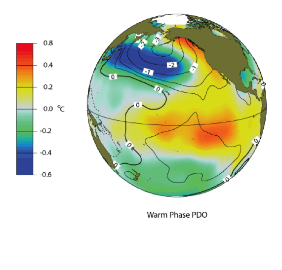
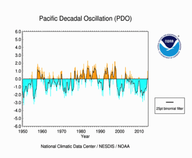
Sea surface temperature pattern showing the warm phase of the Pacific Decadal Oscillation (top). The status of the PDO between 1950 and this year, shown at bottom, indicates a predominantly positive phase from about 1978 to 1998 and negative phase since 1999. Image Credit: Climate Impacts Group, University of Washington.
Footnotes
(1) The degree of predictive skill (or how well the forecasts match with the observations) is often referred to as “predictability.” Skill can be measured in a number of ways and generally indicates the degree to which the forecasts are better than random chance. There is another, more theoretical, definition of predictability that refers to the maximum possible skill under conditions of a huge observational density and accuracy, and tremendously powerful computers to crunch out a forecast from the resulting incredibly mammoth data set. Because of the noise in the climate system such forecasts would still not be perfect.
References
Barnston, A. G., and R. E. Livezey, 1987: Classification, seasonality and persistence of low-frequency atmospheric circulation patterns. Mon. Wea. Rev., 115, 1083-1126.
Dai, A., 2013: The influence of the inter-decadal Pacific oscillation on US precipitation during 1923-2010. Clim. Dyn., 41, 633–646; DOI 10.1007/s00382-012-1446-5.
Livezey, R. E., and M. M. Timofeyeva, 2008: The first decade of long-lead U.S. seasonal forecasts: Insights from a skill analysis. Bull.. Amer. Meteor. Soc., 89, 843-854.
Mantua, N. J., S. R. Hare, Y. Zhang, J. M. Wallace, and R. C. Francis, 1997: A Pacific interdecadal climate oscillation with impacts on salmon production. Bull Amer. Meteor. Soc., 78, 1069-1079.
Thompson, D. W. J., and J. M. Wallace, 2000: Annular modes in the extratropical circulation. Part I: Month-to-month variability. J. Climate, 13, 1000-1016.
Wallace and D. S. Gutzler, 1981: Teleconnections in the geopotential height field during the Northern Hemisphere winter. Mon. Wea. Rev., 109, 784-812.
Comments
I love reading these blogs
Typo?
RE: Typo?
Great catch! The caption should read degrees F. per ten years and not C. We will change it to reflect that. As for the merits of the metric system, I will just say that, personally, I find it much easier to deal with.
Minor, but important correction
Keep up the good work
I've been reading a number of your posts recently, and have learned a fair amount about climate and weather from them (in particular, how complex Earth's climate is). As well, they're really interesting.
Keep up the good work!
Comments have been disabled on this article